Now that we've played with basic math calculations, let's take a
look at some of the basic built in functions available in Excel.
Functions are pre-defined math formulas available in Excel. We're
going to look at the SUM, AVERAGE and ROUND functions.
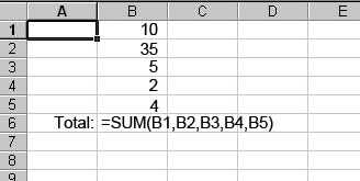
The SUM function adds the cells specified. The format of the SUM
function is =SUM(number1,number2,number3, etc.). The following
are examples of the SUM function:
SUM using each cell address
You can also specify a range of cell addresses to
SUM
Using a COLON (:) between cell addresses tells Excel to use all cells
in the range.
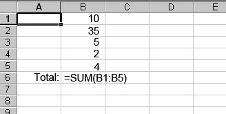
This will add together the values in cells B1, B2, B3, B4 & B5
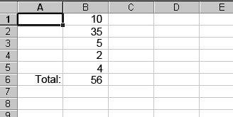
Pressing the ENTER key will display your result
You can use functions by entering them in a cell directly or by
choosing the Functions from the Insert > Functions > Math
& Trig Functions menus. For adding a range of numbers in a
column or row where there is no gap in the data, you can also use
Excel's Auto Sum  function.
Two other commonly used functions are AVERAGE and ROUND.
The format of the AVERAGE function is the same as the SUM function,
i.e., =AVERAGE(number1,number2,number3, etc.) or =AVERAGE(first_cell_address:last_cell_address).
So to calculate the average of the data shown above, you could use
either =AVERAGE(B1,B2,B3,B4,B5) or =AVERAGE(B1:B5)
The format of the ROUND function looks a little different: =ROUND(number,number
of places to round). The number of places to round is specified as a
negative number if rounding to the left of the decimal place and
positive if rounding to the right of the decimal place. For example,
to round 35 to the nearest 10, you would enter =ROUND(35,-1) which
would calculate the result of 40. To round .35 to the nearest 10
cents, you would enter =ROUND(.35,1) which would calculate the result
of .40. To recap:
Round to the nearest 10: =ROUND(number,-1)
Round to the nearest 100: =ROUND(number,-2)
Round to the nearest 1000: =ROUND(number,-3)
Round to the nearest 10,000: =ROUND(number,-4)
Got it? Let's practice. Open
Microsoft Excel and do the following:
-
Start a new
workbook and create a spreadsheet similar to the one below -
replace January xx with the actual dates you will be in
computer class during January starting with today. Using the Page Setup > Custom
Header option, put the title My Typing Speed and your name
in the header. We will be using this throughout the month to enter
typing speed tests results (adjusted WPM) and to calculate our
average typing speed. Save this as YourName - Excel-Typing
| Date |
Calculated Speed (Adjusted WPM) |
| January xx |
|
| January xx |
|
| January xx |
|
| January xx |
|
| January xx |
|
| January xx |
|
| January xx |
|
| Average Typing Speed: |
The formula to calculate your average speed
should go in this cell. |
Now, go and do a Typing Speed Test at FreeTypingGame.net
- Use one of the Classic Tales and do a 2 minute test. Record the Calculated
Speed (which is adjusted WPM) next to the correct date. Remember this
is a speed test so don't look at your hands; it will only slow you
down! If you can't help yourself, use one of the keyboard shorts to
cover your hands. The first thing you should do when you get to
class every day in January is to open this Excel workbook and take
your typing speed test for the day!
- Using
the numbers below, find the sum of all of the numbers, the average
of all of the numbers and round each number to the nearest 10,
100, and 1000. Use the SUM, AVERAGE & ROUND functions to do
these calculations. Save this as
YourName - Excel4.
| 85654489 |
579237295 |
73245648 |
85753638
|
7543790 |
Back to Computer
Lab

